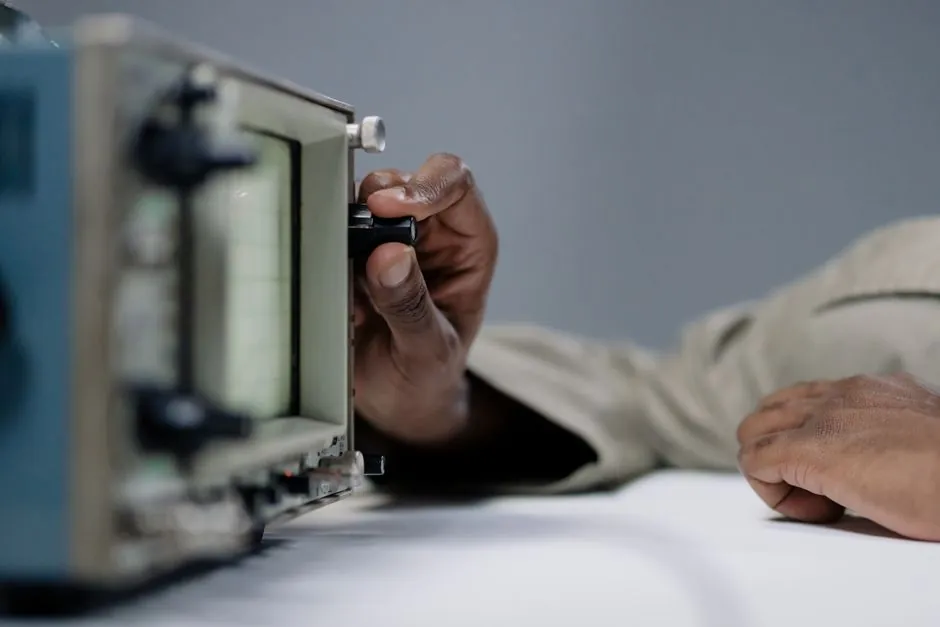
A brick-wall (maximally flat) oscilloscope response holds amplitude close to unity from DC to roughly 80% of the rated -3 dB bandwidth, then attenuates sharply above it, while a Gaussian response rolls off smoothly from well below the -3 dB point [S1][S5].
At the same nominal 1 GHz bandwidth, the two shapes give measurably different rise-time constants, different aliasing risk on a digitised scope, and different error when the probe, fixture, or source adds its own bandwidth to the measurement chain [S1][S3][S5].
Defining the Two Response Shapes
A Gaussian frequency response is the cascaded behaviour of many similar, gentle analogue stages, and is typical of traditional analogue oscilloscopes and of many sub-2 GHz digital scopes [S1][S5]. Its magnitude plot is a single-pole Gaussian curve, attenuated by 3 dB (70.7% of input amplitude) exactly at the rated bandwidth frequency [S5].
A brick-wall response, also called maximally flat, is flat to within a small percentage of unity across most of the passband and then falls off steeply past the rated bandwidth [S1][S3]. It is implemented in real-time digital scopes by combining a small number of analogue stages with DSP magnitude-flattening and phase-correction filters [S1][S2].
True hardware brick-wall filtering at, say, 10 GHz is not physically realizable, so modern scopes approximate it with a hardware roll-off that the FIR filter then sharpens in the DSP domain [S2].
Rise-Time Constant: k = 0.35 vs k = 0.40 to 0.45
The standard step-response rule rise time = k / bandwidth applies to both shapes, but with different k values: k = 0.35 for a Gaussian system, and roughly k = 0.40 to 0.45 for a brick-wall (maximally flat) response [S1][S5].
That difference is the opposite of what most first-time buyers assume. A 1 GHz Gaussian scope is rated around 350 ps rise time, while a 1 GHz brick-wall scope of the same nominal bandwidth measures closer to 400 to 450 ps on a fast edge [S1][S5].
Total system bandwidth in a Gaussian architecture combines as the root-sum-square of the individual stage bandwidths, so adding a faster probe or preamp does not proportionally improve the figure, which is why the probe bandwidth is usually kept at or above the scope bandwidth [S1].
Measured rise time combines signal and scope in quadrature: T_measured = sqrt(T_signal^2 + T_scope^2), which is only valid when the scope rise time is not dramatically faster than the signal edge, otherwise the formula under-corrects the de-embedding step [S1].
Where Each Response Excels, and Where It Fails
Gaussian response is the right choice when pulse fidelity matters more than raw amplitude accuracy: a step into a Gaussian scope never overshoots, regardless of how fast the input edge is, because there are no passband ripples to ring [S1][S4].
Brick-wall response is the right choice for amplitude-accurate work on sinewaves, modulated carriers, and spectrum-sensitive measurements, because the in-band amplitude is flat to within 1 to 2% instead of drooping several percent as you climb toward the -3 dB point [S1][S3].
For digital-bus work, the rule of thumb is to pick scope bandwidth at 2.5 times the bit rate, so that the fifth harmonic of a 1 Gb/s signal sits at 2.5 GHz inside the passband; this ratio only gives clean eye diagrams if the response is flat to that frequency, not drooping toward it [S5].
Brick-wall response also reduces sampling-aliasing errors on a real-time digitising scope, because out-of-band content past the steep roll-off is strongly attenuated before the ADC sees it, so the Nyquist zone is cleaner [S1][S2].
However, a brick-wall passband is a poor match for applications whose primary object of interest is the rise time of a pulse rather than its amplitude: the steeper magnitude slope and altered phase behaviour distort edges more than the gentle Gaussian roll-off [S4].
Decision Comparison at the Same Nominal Bandwidth
Below is the practical contrast at, for example, a 1 GHz scope, drawn directly from the cited response-shape references. [S1]
Amplitude accuracy in passband: Gaussian rolls off gradually, reaching about 2% attenuation at roughly 20% of rated bandwidth, so a 200 MHz signal on a 1 GHz Gaussian scope is already down ~2% [S5]. Brick-wall stays within roughly 1% out to 80% of the rated bandwidth [S1][S3].
Rise-time constant: k = 0.35 (Gaussian) versus k = 0.40 to 0.45 (brick-wall) in the rise time = k / bandwidth formula, so brick-wall is slower on a fast edge at equal nominal bandwidth [S1][S5].
Pulse overshoot: Gaussian is monotonic, no overshoot on any step input; brick-wall can show passband-related ringing on very fast edges because of the steeper magnitude transition [S1][S4].
Aliasing exposure for real-time scopes: Gaussian lets more out-of-band content through to the ADC; brick-wall attenuates it before digitisation, so a DSP-flattened scope is the better host for single-shot capture at high time-base settings [S1][S2].
How DSP Closes the Gap
Modern high-speed real-time scopes apply five classes of DSP filtering to the acquired record: waveform reconstruction (sin(x)/x or linear), magnitude flattening, phase correction, noise reduction, and bandwidth enhancement [S2].
Magnitude flattening and phase correction are exactly the two stages that turn a near-brick-wall analogue front end into a true maximally-flat passband, and they run in a single FIR filter per acquisition [S2].
Waveform-reconstruction filtering is what interpolates between 50 ps sample points on a 20 GSa/s scope, and sin(x)/x is the accurate choice only when no signal energy sits above the Nyquist frequency, which is why the hardware analogue roll-off must precede the ADC in the first place [S2].
The same DSP path that flattens a brick-wall response is also what lets scope vendors publish bandwidth figures close to the brick-wall cut-off rather than the more conservative Gaussian cut-off at 1 GHz and above [S3].
Implications for Spec Writers and Buyers
If the spec demands amplitude accuracy better than 2% on signals that approach 50 to 80% of the scope's rated bandwidth, write the requirement as a brick-wall or maximally-flat response, not as a generic "1 GHz bandwidth" line item [S1][S3].
If the spec is for clean pulse edges with no overshoot, write it for a Gaussian response and accept the k = 0.35 rise-time constant, because the brick-wall shape trades edge fidelity for in-band flatness [S1][S4].
Always combine the scope, probe, and fixture bandwidths as the root-sum-square when computing system rise time, and oversample at 2.5 to 5 times the scope bandwidth to keep the ADC honest on single-shot captures [S1][S5].
Watch the next signal: vendor datasheets increasingly quote "flat bandwidth" as a separate spec from "Gaussian equivalent bandwidth" on 1 GHz-plus scopes, so the gap between the two rise-time constants is becoming a line item in its own right.
Detailed specification references: diaphragm wall grab, glass curtain wall, and door window curtain wall.
For related coverage, see Selecting a Flow Meter for High-Viscosity Chemical Fluids: PD vs Coriolis vs Alternatives.