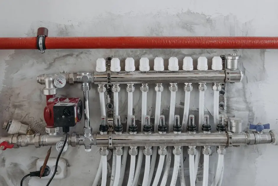
A defensible pressure-transmitter total probable error calculation converts reference accuracy, ambient-temperature effects, static-pressure effects, calibration uncertainty, drift, and installation errors into a common unit, typically % of calibrated span [S3][S4].
The result estimates installed performance across defined operating conditions, and it is more useful for calibration planning than laboratory accuracy alone [S2][S7].
TPE scope and required performance
Total probable error is a combined estimate of how far an installed pressure measurement may differ from actual process pressure under stated conditions [S4]. Reference accuracy covers non-linearity, hysteresis, and non-repeatability under laboratory or reference conditions, while installed performance adds ambient-temperature variation, elevated static pressure, and other application effects [S3].
A defensible accuracy budget should state a consistent basis, such as percent of calibrated span, and separate reference accuracy from temperature effects, calibrated-span or turndown effects, calibration uncertainty, drift, and installation-specific residual errors [S4].
Begin with the pressure type, normal, minimum, and maximum pressure, calibrated range, upper range limit, ambient range, process temperature, static pressure, required calibration interval, and the governing decision tolerance [S4]. A pressure transmitter calculation is valid only for the stated calibration span and operating envelope.
Build the calculation in one common basis
Convert every error contribution to psi, bar, kPa, or a percentage of calibrated span before combining them [S4]. A 0–100 psig transmitter with ±0.10% calibrated-span accuracy has a ±0.10 psi reference limit; ±0.10% of URL also equals ±0.10 psi when URL is 100 psi, while ±0.10% of reading equals ±0.05 psi at 50 psi [S4].
Use this conservative arithmetic budget when the manufacturer provides individual limits but does not define a statistical combination:
<strong>TPE = reference accuracy + temperature effect + static-pressure effect + calibration uncertainty + drift + residual installation error</strong> [S3][S4].
Worked example: for a 0–100 psi transmitter, add ±0.10 psi reference accuracy, ±0.20 psi temperature effect, ±0.15 psi static-pressure effect, ±0.05 psi calibration uncertainty, ±0.10 psi drift, and ±0.05 psi residual installation error. The conservative TPE is ±0.65 psi, equivalent to ±0.65% of calibrated span [S4]. If a method combines independent uncertainties statistically, document the distribution assumption and do not describe the result as a worst-case limit [S4].
Compare the main error methods

Reference accuracy is specified under controlled conditions and is not an installed-performance result [S3][S4]. A manufacturer calculation tool can apply model-specific coefficients for temperature, head effect, static effect on zero, and response time, with a printable report structure, but its default model data and assumptions must be checked before reuse [S1].
Do not mix percentage of URL, percentage of calibrated span, and percentage of reading inside one budget without conversion [S4]. Manufacturer definitions of TPE are not uniform, so compare the included effects and statistical treatment rather than comparing headline numbers alone [S4].
Diagnose the dominant contributors
<strong>Symptom: error grows with ambient-temperature change.</strong> Root cause: the transmitter is operating away from its reference temperature, or the selected range is not compensated for the service temperature. Corrective action: obtain the temperature coefficient from the model datasheet and calculate the error at minimum and maximum ambient conditions. Accept the installation only if the combined TPE remains below the application tolerance [S2][S4].
<strong>Symptom: differential-pressure error grows with static line pressure.</strong> Root cause: static pressure shifts the sensing element or introduces a span effect. Corrective action: add the manufacturer's static-pressure effect at the maximum operating pressure and test at the differential pressure of interest; do not reuse a low-static-pressure result [S2][S3].
<strong>Symptom: zero error increases after a line-pressure excursion.</strong> Root cause: zero shift or static effect on zero. Corrective action: include the static zero contribution, perform a pre- and post-test zero check, and replace or recalibrate when the shift exceeds the assigned TPE or control tolerance [S1][S4].
<strong>Symptom: calculated error rises after a range or calibration change.</strong> Root cause: reference accuracy is being applied to the wrong basis, or zero and span errors were not separated. Corrective action: confirm LRV, URV, URL, and configured span, convert each specification to % of calibrated span, and rerun the budget [S4].
Apply installation and verification controls
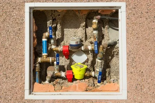
Residual installation error can include inaccessible tapping points, liquid-filled impulse lines, elevated or restricted mounting position, process-media density effects, and unresolved zero or range offsets [S3][S4]. Record mounting position, impulse-line configuration, process and ambient conditions, and the orientation used for calibration.
Use a pressure calibrator with uncertainty adequate for the assigned acceptance limit, and verify at the zero, span, and intermediate points that matter to the process. For a differential transmitter, include high- and low-pressure sides and the applicable static-pressure condition. For a gauge, absolute, or level measurement, use the corresponding reference type and apply the correct tap-pressure correction [S4].
Escalate rather than adjust when the observed error exceeds the calculated TPE, the tap or impulse-line condition is unstable, or the calibrator uncertainty is a significant fraction of the acceptance tolerance. A zero adjustment can mask a failed sensor or unsuitable installation and should not be treated as proof that the original budget is valid [S4].
Convert TPE into a calibration interval
A transmitter with a smaller calculated TPE can generally support a longer interval, but TPE alone does not set the interval [S2]. The method begins with required performance and operating conditions, calculates TPE, identifies output-stability specifications, and then calculates calibration frequency [S2].
Use calibration history to establish drift and repeatability at the chosen interval. For differential-pressure transmitters used in flow applications, 40 CFR Part 98 recommendations call for annual recalibration or the minimum manufacturer-specified frequency [S2]. This regulatory reference does not replace a plant-specific calculation based on stability, drift, and required installed performance [S2].
Record the model code, serial number, calibrated span, URL, reference accuracy, temperature and static-pressure coefficients, calibration uncertainty, observed drift, TPE, and next review date. ABB's Pressure Total Performance Calculator provides inputs for temperature data, head effect, static effect on zero, and response time, while its model-specific output should be checked against the installed conditions [S1].
Set the next review trigger as either the planned date or an early inspection when measured drift approaches the remaining TPE budget, with the application tolerance providing the final acceptance criterion [S2][S4].
The practical checkpoint is a signed accuracy budget in one unit and one basis: if a field check cannot be traced to LRV, URV, URL, operating temperature, static pressure, and calibrated span, the calculated TPE is not auditable.