
An LCR meter may show readings more than 20% away from the expected value when the test frequency, impedance model, or source condition is unsuitable [S1].
The accuracy chart must be read as a combined specification covering impedance magnitude, frequency, percentage of reading, test level, and fixture or calibration errors, not as one universal accuracy statement [S1][S3][S4].
Accuracy chart coordinates and operating conditions
An LCR meter determines complex impedance from voltage, current, and phase angle, so an accuracy curve normally needs an impedance axis, a frequency axis, and a defined error expression [S2][S4]. For a fixed component model, the horizontal axis represents impedance magnitude and the vertical axis represents the permitted error, while the constant-C and constant-L loci appear as diagonal reference lines [S4].
The frequency attached to each curve changes the component under test, not just the instrument setting. Capacitive reactance is \(X_C=1/(2\pi fC)\), while inductive reactance is \(X_L=2\pi fL\); therefore the same physical component can cross several impedance ranges as frequency changes [S5]. A reading outside the charted impedance and frequency domain has no supported accuracy claim, even if the displayed value looks stable [S1][S4].
Check the test level as well as frequency. The generated signal voltage should match the circuit's normal operating voltage because both the accuracy and stability of that signal vary by instrument [S2]. Open-circuit voltage mode is recommended for ordinary objects with average impedance, while constant-current mode gives more stable readings for inductors [S1].
Percentage of reading versus percentage of range
A percentage-of-reading error applies directly to the displayed value, while a percentage-of-range error is calculated against a stated full-scale quantity, so the two forms must not be compared as equivalent limits [S1][S4]. Interpret the formula printed beside the plot, including whether the chart expresses accuracy as a positive or negative tolerance, because the permitted measurement interval can be centered on the nominal value or bounded asymmetrically.
For example, a curve specified as ±1% of reading at 100 Hz supports a 100 ohm result of 99 to 101 ohm, while a ±1% of full-scale specification over a 1 kilohm range permits a much wider result interval. The chart must also identify any additive term, because a specification such as percentage of reading plus a fixed number of ohms produces a nonlinear absolute-error band across the impedance range [S1][S4].
Do not treat the plotted point as a guarantee for every equivalent circuit. The meter applies a Thevenin equivalent at its terminals, and real loads combine resistance with capacitive or inductive reactance; series and parallel models can yield different derived L, C, R, ESR, or Q values from the same measured impedance [S1]. The AC bridge measurement method explains how that terminal equivalent is measured.
Choosing the appropriate instrument method
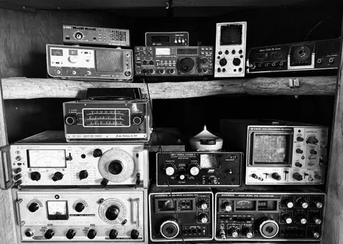
An LCR meter is suitable for repeated component measurements where test frequency, signal accuracy, and stability dominate instrument selection, with 1 kHz and twice the line frequency identified as useful operating points in the cited guide [S2][S6]. It can also report phase angle, dissipation factor, reactance, conductance, susceptibility, quality factor, and equivalent series resistance, while a basic digital multimeter normally does not provide the same phase-sensitive component characterization [S2].
An impedance analyzer becomes the stronger choice when parasitics, fixture effects, or transmission-line behavior dominate the result. Auto-balancing-bridge LCR meters are generally suited to lower frequencies, whereas RF current-voltage or network-analysis analyzers extend usable coverage into higher frequency ranges [S3]. The comparison spans 1–100 MHz and identifies LCR degradation beyond 1 MHz, along with analyzer calibration and transmission-line effects, as high-frequency concerns [S3].
For broad sweeps, nonlinear frequency response, or device characterization beyond discrete L, C, and R values, an impedance analyzer provides the more defensible workflow. For production testing of ordinary inductors, capacitors, and resistors at controlled frequencies, the LCR meter is usually faster and less demanding [S2][S6].
Fixture, calibration, and error contributors
High-frequency accuracy depends on calibration discipline, but even a calibrated instrument can lose accuracy through stray capacitance, lead inductance, impedance discontinuities, and fixture parasitics [S3]. Calibration removes a defined set of system errors; it does not correct an unstable DUT, a poorly seated component, or an unsuitable equivalent-circuit model. Record open, short, and load compensation status before using a charted limit in production or engineering comparison [S3][S4].
De-embedding is only valid when the fixture model and the physical connection are controlled. The cited high-frequency comparison identifies transmission-line effects and calibration as concerns and does not state specific 10 MHz or 30 MHz thresholds or discuss variable de-embedding effectiveness [S3]. These boundaries make physical separation, lead arrangement, fixture repeatability, and stabilization time part of the accuracy budget, not incidental setup details.
Measurement speed also affects usable accuracy. Response time is the interval required for a stable displayed result, and some instruments shorten it by reducing measurement quality; a production test that accepts the first reading can therefore be less repeatable than a slower verification cycle [S2]. Set averaging or trigger conditions explicitly and record them with the result.
Decision table for practical verification

The correct selection rule is to map the DUT to an impedance and frequency region, select a chart whose axes cover that region, then verify the complete error budget. A 1 kHz reading does not establish performance at 10 MHz, and a 20% result cannot be defended by quoting a percentage-of-range specification that applies only near full scale. [S3]
For a practical comparison, a basic LCR meter offers the lowest setup burden for discrete R, L, and C checks at specified frequencies, but its useful accuracy is bounded by fixture and frequency effects [S1][S2]. An auto-balancing-bridge LCR meter adds precision for impedance and phase work, although degradation beyond 1 MHz and parasitic effects remain concerns [S3]. An RF impedance analyzer offers wider frequency coverage and better fixture or de-embedding options, at the cost of greater calibration complexity above 10 MHz [S3]. A data logger can preserve stabilized results, but it does not remove uncertainty from the measurement chain.
Use the strictest applicable boundary when multiple contributions exist: the lower frequency limit of the chart, the nearest impedance limit, the specified test current or voltage, the DUT's series or parallel model, and the calibration state. A result is defensible only when all five conditions are documented and the observed value, including the chart's tolerance and any offset, remains inside the calculated interval.
Acceptance workflow for component data
A controlled LCR measurement should record the instrument model, serial number, calibration date, fixture identity, test frequency, test level, equivalent-circuit mode, stabilization rule, and raw complex result before conversion to L, C, R, ESR, or Q. At 1 kHz and twice the line frequency, separate curves may be needed because the same component can occupy different impedance points on each chart [S6].
Flag every reading outside the published impedance or frequency envelope instead of applying a generic tolerance. Measurements above 30 MHz require explicit attention to thermal drift, while measurements above 10 MHz require review of calibration, transmission-line effects, and de-embedding [S3]. For inductor stability, constant-current operation is the defensible selection when comparing repeated readings [S1].