A process calibrator simulates a thermocouple by replacing the sensor with a stable, low-impedance DC millivolt source that outputs the exact thermoelectric voltage the thermocouple would produce at the selected hot-junction temperature [S1][S4]. The technician dials in a type and a temperature (for example, Type K at 600 °C), and the instrument synthesises the corresponding mV from internal tables derived from the published type-specific characteristic curves [S4][S5].
This decouples the controller, transmitter, data logger, or PLC input from the physical sensor so the electrical side of the thermocouple chain can be checked step by step, without heating the process or pulling a probe out of service [S4].
What the mV signal actually represents
A thermocouple generates a small DC voltage proportional to the temperature difference between its measuring junction and its reference (cold) junction, with most common types sitting in the millivolt range across their useful span [S4]. A Type K sensor, for example, produces about 4.096 mV at 100 °C and roughly 24.995 mV at 600 °C against a 0 °C reference, so a calibrator simulating Type K at 600 °C has to deliver the same ~24.995 mV to its terminals [S4].
Because the output is referenced to a fixed internal 0 °C compensation point inside the calibrator, the instrument is essentially playing the role of a "perfect thermocouple" sitting on a bench at 0 °C with a hot junction at the user-set temperature [S4][S5]. Devices that also include a millivolt source/measure mode let the user drive a raw mV value (for example, 10.000 mV) directly, which is the same signal expressed without the thermocouple-type wrapper [S5].
How the instrument generates the voltage internally
Inside a handheld process calibrator the synthesised thermocouple signal comes from a precision low-noise DC reference (typically a band-gap or DAC-driven reference) that is scaled and offset by low-drift amplifiers and a precision resistor network to produce the microvolt- to millivolt-level output [S2][S5]. The selected type and temperature are converted through an internal polynomial or lookup table derived from the relevant IEC 60584 type tables, and the resulting target mV is fed to the output terminals through a low-impedance buffer so the device under test does not load the reference [S4][S5].
Output ranges for handheld mV source typically sit in single-digit millivolts to around 100 mV (the 1586A Super-DAQ, for example, is specified at -15 mV to 100 mV with 0.004% + 4 µV accuracy, while the 1560 Black Stack covers -10 to 100 mV at ±0.002 mV), and dedicated thermocouple sources extend that to roughly ±100 mV with microvolt resolution [S1]. Typical multifunction calibrator accuracy in this range is around 0.05% of reading for mV and mA, dropping to 0.01% on more expensive bench units [S1][S5].
Why a technician uses simulation rather than a real sensor
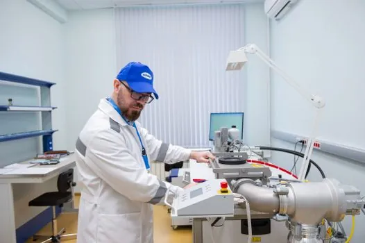
Simulation is the standard way to fault-isolate a temperature loop: if the controller reads the set value while driven by the calibrator, the input, parameterisation, terminals, and cold-junction compensation are working, and the problem is downstream (sensor, sheath, installation) or in the process itself [S4][S6]. If the controller reads wrong during simulation, the cause is in the evaluation side: wrong input type selected, bad cold-junction compensation, swapped polarity, or a damaged compensator lead [S4].
The same technique verifies a thermocouple transmitter's 4-20 mA output by stepping the simulated mV through zero, working range, and full scale and watching the loop current, which is a typical field workflow on power-plant and furnace instrumentation [S4][S6]. Where a multifunction process calibrator is available, the same instrument that simulates the thermocouple can also read the 4-20 mA loop and power it, so the entire input-plus-transmitter branch is checked from one box [S1][S5].
Common thermocouple types and their working ranges
Handheld calibrators typically support the popular base-metal types (J, K, T, E) plus the noble-metal types (R, S, B), and the better units extend coverage to N, L, U, C, G, D, P, M, and the Russian/Brazilian XK and BP variants [S1]. The published working envelopes for the Fluke 724, 725, 726, 7526A, and 754 all cluster around -200 °C to +1800 °C, with the 714B thermocouple-only calibrator covering -250 to +1410 °C across 17 types [S1].
Comparing the main options on three decision criteria:
1. Coverage vs cost. A dedicated thermocouple calibrator (Fluke 714B) gives the widest type list (17 types, -250 to 1410 °C) at the lowest price; a multifunction calibrator (725/726) trades some type breadth for mA, mV, RTD, and loop-power in one box; a bench precision unit (7526A) gives the best accuracy over -250 to 1767 °C across 14 types but at significantly higher cost [S1].
2. Accuracy. Handheld mV source is typically 0.05% of reading; bench and documenting units push to 0.004% + 4 µV on the 1586A Super-DAQ or ±0.002 mV on the 1560 Black Stack, which is the difference between a 0.5 °C and a 0.05 °C equivalent at Type K 600 °C [S1].
3. Workflow. A handheld simulator is the right tool for in-cabinet loop checks and fault isolation; a dry-block or furnace comparison calibration with a reference PRT is required when the goal is a traceable statement of the sensor's own accuracy, not just the loop's behaviour [S1][S3].
Cold-junction compensation and the simulation boundary
Simulation only checks the electrical evaluation side of the signal calibrator chain, not the sensor itself, and that boundary is the whole point of the technique [S4]. A real thermocouple also requires cold-junction compensation inside the readout or transmitter, because the device has to back out the temperature of the reference terminals; when a calibrator simulates the thermocouple, the calibrator's own internal reference acts as the 0 °C reference, so the DUT's CJC only adds its own error on top of an otherwise perfect signal [S3][S4][S5].
For traceable sensor calibration, this is the limitation that pushes users toward comparison methods: a reference PRT, a stable heat source, and a documented read-out, producing the deviation at chosen test points with a chain of evidence back to national standards [S1][S3]. A prior calibration result is a status backed by paperwork, not a permanent property of the sensor, and a thermocouple's thermoelectric state can change with temperature exposure, so the process control loop should be re-validated on a risk-based interval rather than on a calendar guess [S3].
Limitations, common errors, and what simulation does not catch
A simulation cannot detect a sensor that has drifted, a junction that has shorted to ground, an open sheathed probe, or a degraded extension/compensating cable, because the calibrator has replaced the sensor entirely [S4]. It also cannot verify whether the thermocouple type configured in the controller matches the physical type wired in, only whether the configured type reads correctly when fed the matching simulated signal [S4].
Field failures that simulation routinely catches, by contrast, include wrong input type (controller set to Type J but field wired as Type K), reversed polarity at the terminals, CJC disabled in software, and a transmitter whose 4-20 mA loop is scaled for a different range, all of which show up immediately when the calibrator drives 0%, 50%, and 100% of span [S4][S6]. Some calibrators add a secondary millivolt display alongside the temperature readout, so the technician can confirm the actual mV being delivered matches the expected mV for that type and temperature, which closes the loop on whether the calibrator itself is doing the maths correctly [S8].
Two trackable signals to watch: (1) the migration of documenting multifunction calibrators (Fluke 754, 726) into HART- and Ethernet-APL-capable temperature loops, where the same instrument now sources the thermocouple mV and configures the smart transmitter in one pass, and (2) the continued split between simulation-based loop verification (fast, electrical-only) and comparison-based sensor calibration (slow, traceable, with reference PRT) as separate disciplines that answer different questions on the same measurement chain [S1][S3][S4].
Background reading: Duty Drawback for Re-Exported Industrial Equipment: 2026 Rules and Filing Traps.