
Fast I/O on a modern machine is not won by picking the fastest CPU; it is won by budgeting the whole response path, with task execution under 10 ms, end-to-end latency under 2x worst-case scan, and an explicit safety margin below the watchdog [S3][S1].
For packaging, sortation, and safety circuits, the four-step PLC cycle (input scan, logic execution, output update, housekeeping) repeats hundreds of times per second, and a missed signal can mean a timing error or a real hazard [S2][S1]. Designers who plan for a single scan are surprised; designers who plan for two scans are rarely late [S4].
Anatomy of the Scan and Where the Budget Leaks
Total scan time is the sum of four contributors: program execution, I/O processing, communications, and housekeeping, and the canonical formula is T_scan = T_program + T_I/O + T_comm + T_housekeeping [S1]. In the FIRGELLI estimator, a 64-point, 250-rung, 2-comm-module configuration returns 1.06 ms scan and 2.13 ms worst-case response, roughly doubling the scan as the practical input-to-output ceiling [S1].
Two rules of thumb separate the textbook from the machine floor: the longest possible input-to-output delay can reach 2x scan time when an input arrives just after the input scan, and high-volume discrete cells add one full cycle of "green light wait" between every sequential step [S4]. A six-step, 30-second machine running 8 hours a day on a 30 ms scan loses about 2,250 parts per year versus a 6 ms scan, around 2.25 million dollars per year at a $1,000 part price, which is why two-scan budgeting is the default for production accountants [S4].
Scan Time vs. End-to-End Response: The Gap Most Specs Miss
Scan time describes only the logic-execution portion of the path, while the field response includes module update, task wait, output update, and device actuation, and confusing the two is the single most common timing failure on commissioned cells [S3]. On a 10 ms periodic task, a vendor monitor will report last execution (2.6 ms), average execution (2.3 ms), maximum execution (4.4 ms), and a 20 ms watchdog, each value serving a different engineering purpose and none of them interchangeable [S3].
Hardware interrupts break the scan ceiling entirely: a fast input can trigger an interrupt service routine that fires in microseconds, decoupled from the cyclic task, which is why "fast response times do not equal fast scan cycles" is the headline finding for designers sizing motion and safety paths [S6]. The full response path is physical input, module update, wait for task, execute logic, output update, and device, and that string must be measured end-to-end when the requirement is safety- or process-critical [S3].
Choosing a PLC Family by Timing Profile, Not Brochure
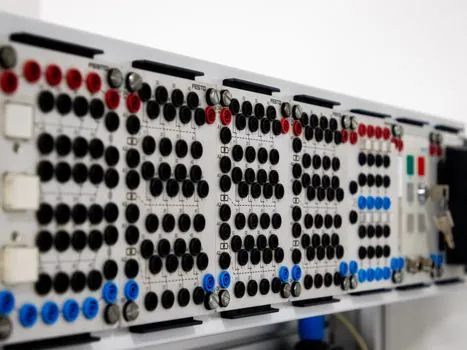
Selecting the fastest PLC means comparing scan time, bit-instruction execution, analog conversion, and I/O filter response as a stack, because a 1 ms CPU with a 5 ms analog input filter still cannot close a 2 ms loop [S5]. Compact, modular, safety, and motion controllers each carry different scan signatures: safety PLCs add deterministic diagnostics overhead, while motion controllers drop scan to sub-millisecond but require matched servo cycle budgets, see the PLC control reference for the architectural differences that drive those numbers.
Platform terminology also matters: Rockwell Studio 5000 exposes LastScanTime and MaxScanTime on the Program and Task objects, Siemens STEP 7 reports cycle time and OB runtime with previous, minimum, and maximum values on S7-300/400 OB1, and CODESYS separates last/average/max cycle time from periodic jitter in the Task Configuration monitor, so the diagnostic tag you read on day one is not the same on day two if you change platform [S3]. An automation cell that needs a single I/O event to land inside one cycle should budget that event against the PLC maximum observed scan, not the average, and keep the watchdog out of the design margin [S3].
Distributed I/O, Asynchronous Updates, and the Jitter Problem
Distributed I/O updates asynchronously to logic, so a fast task alone does not guarantee a fast field response, and a 1 ms scan on the controller can sit behind a 4-8 ms PROFINET or EtherNet/IP update window on the slice [S3]. The mitigation is to set the task period to the I/O update interval you actually have, not the one you wish you had, and to verify the configuration with vendor tools on the target firmware.
For a guide to see how a safety PLC layers its own watchdog and proof-test interval on top of the cyclic scan, the dedicated reference covers the diagnostic-rectangle logic and the safety reaction time that sits beside, not inside, the standard scan budget. The headline rule is that a watchdog is a fault boundary, not a design target: normal worst-case execution needs deliberate margin below it, and reset-and-observe over startup, production, faults, recipes, and communication bursts is the only way to capture the maximum that matters [S3].
Measurement Checklist Before the Machine Ships

A timing result is only credible when it is logged with controller model, firmware, task type, priority, period, and watchdog on the same line as the scan number, because a "6 ms scan" without context is unfalsifiable on a different CPU [S3]. Reset the diagnostic counter, run the cell through startup, normal production, a fault, a recipe change, and a communication burst, and read the maximum execution, not the last, for the deadline review [S3].
Where the response requirement is in the 1-5 ms range, the same checklist must include the physical input-to-output path, including sensor debounce, module filter setting, network update, output module turn-on, and actuator stroke time, because any one of those can dominate the scan itself. As a related sizing case on a different but adjacent problem, sizing a pneumatic cylinder for 500 N push: bore, stroke, and safety margin walks through the same kind of "sum the contributors, then add margin" budgeting that scan-time work demands, and the MG1 Part 30 vs Part 31 motor on a general-purpose VFD: spec, insulation, and risk cross-walk shows the same pattern of stacking manufacturer-specific cycle numbers against an application deadline.
Decision Matrix: Which Lever Closes the Gap
Three levers actually shrink input-to-output latency on a shipped machine, and they are not interchangeable: tighten the cyclic scan (faster CPU, slimmer program), shorten the task period (move the event to a higher-priority task), or break the scan entirely with a hardware interrupt or dedicated I/O module [S6][S3]. On a 6-step, 30-second machine, dropping scan from 30 ms to 6 ms recovered about 2,250 parts per shift per year, more than any one-time mechanical tweak available to the cell [S4].
Use the matrix below to pick the lever against the symptom you actually have on the bench.
Symptom: occasional missed pulses, fast inputs not seen. Fix: enable a hardware interrupt on the input module, accept microsecond-class response independent of scan. Best when the pulse is shorter than one scan and counts matter [S6].
Symptom: average response acceptable, but worst-case tail too long. Fix: tighten the program, split tasks by priority, and budget maximum scan below the application deadline with margin. Best for serial production cells with 6+ sequential steps [S4][S3].
Symptom: scan looks fine in the monitor, but field device responds late. Fix: measure the full physical path and resync the task period to the distributed I/O update window. Best for cells with PROFINET or EtherNet/IP slices at 4-8 ms update [S3].
For motion-centric builds, the time relay reference covers the deterministic timing primitives that often sit beside the scan loop, useful when off-scan sequencing is the right architectural answer.
Limits, Failure Modes, and What to Verify

Three failure modes recur on commissioned machines: treating scan as the full response path, treating the last or average scan as the worst case, and letting the watchdog creep toward the operating point during a recipe change [S3]. The published six-month guidance from plcprogramming.io, cross-checked against Studio 5000 V38, STEP 7 V21, and CODESYS task-monitor documentation, recommends capturing last, average, maximum, interval, jitter, and watchdog on the target controller, not a generic brochure [S3].
The historical Schneider Electric data point is also worth keeping: a 6 ms scan upgrade on a six-step, 30-second machine added about 120 engines per day in a documented engine plant retrofit, and the same order-of-magnitude gain has been repeated on similar discrete cells when the scan was the binding constraint [S4]. When the binding constraint is instead I/O filter time, network update, or actuator stroke, no amount of CPU speed will close the gap, which is why a stopwatch measurement of the physical path is the only evidence that matters for a signed-off acceptance test [S3].
Track these two signals going forward: vendor release notes for STEP 7 V21+ and Studio 5000 V38+ that re-baseline task-monitor fields, and any IEC working group update to the program execution concepts that govern how "scan time" is defined across runtimes, because the diagnostic tag names and exposed attributes change between minor versions even when the underlying cycle numbers move only modestly.