
A temperature transmitter that accepts a thermocouple input compensates the cold junction by measuring the temperature of its own terminal block with an onboard semiconductor or RTD sensor, then adding the equivalent Seebeck voltage for that temperature (looked up from NIST type tables) back into the measured millivolt signal so the result equals what the thermocouple would have produced with its reference at 0 °C [S2][S4].
Inside a typical 4-20 mA HART or Foundation Fieldbus head-mount or DIN-rail transmitter the compensation chain runs: thermocouple wires to isothermal terminal block, on-board reference sensor (often a precision silicon diode or Pt100), 24-bit delta-sigma ADC, a microcontroller running polynomial conversions per IEC 60584-1 type tables, then the correction sum, then output linearization to °C or engineering units [S3][S6].
Why a thermocouple cannot read absolute temperature on its own
A thermocouple is two dissimilar alloy wires welded at the measuring (hot) junction, and the open (cold) ends sit at the transmitter terminals. The Seebeck effect generates a voltage proportional to the temperature difference between those two junctions, not to absolute temperature at the hot end, so a Type K with 41.0 µV/K sensitivity [S5] reading a 400 °C process with the cold end at 30 °C produces voltage equivalent to a 370 °C differential; if the system naively assumes 0 °C at the terminals, it underreports by 30 °C [S4].
Standard thermocouple reference tables published under IEC 60584-1 are tabulated against a 0 °C reference junction, which is why the historical laboratory method immersed the cold-end wires in an ice bath; any modern field instrument must electronically rebuild that 0 °C reference [S1][S4].
The four hardware blocks that do the compensation
First, an isothermal terminal block forces both thermocouple legs to track the same temperature, so a single reference-sensor reading represents the cold-junction temperature for both polarities; poor thermal coupling here is the dominant source of gradient error [S2][S3].
Second, an onboard temperature sensor measures the block: classic analog designs used an LM335 with 10 mV/K nominal sensitivity, resistor-factored down to the µV/K range to match the thermocouple's Seebeck coefficient (for example, 898 Ω to match Type K when R3 is 220 kΩ) [S5].
Third, the thermocouple millivolt signal and the reference-sensor signal are digitized by a 24-bit delta-sigma ADC with effective resolution of about 0.02 °C on a Type K input [S3].
Fourth, firmware applies the inverse Seebeck polynomial for the configured thermocouple type to convert the reference temperature into an equivalent millivolt value, adds it to the measured thermocouple voltage, and re-applies the forward polynomial to output °C; this re-uses the standard NIST/ITS-90 coefficient sets per thermocouple type [S6][S7].
Software correction path: from millivolts to compensated °C

The microcyber-fieldbus reference describes the calculation as: the transmitter measures the cold-junction temperature T_cj at any moment, looks up the corresponding thermocouple voltage V_cj from the type table, and adds it to the measured hot-junction voltage V_meas, so the total V_hot = V_meas + V_cj can be inverted through the same table to give T_hot as if the reference were at 0 °C [S6].
Texas Instruments' SLOA204 walks through the same chain in analog form: the LM335 voltage is scaled by a resistor divider (R4 = α / 10 mV * R3) so the 10 mV/K output of the sensor matches the 40.8 µV/K of Type K, then a zener-derived offset of about 2.73 V is subtracted so that at 0 °C the output reads zero, which is the analog equivalent of the digital table-lookup [S3][S5].
Accuracy budget, ambient limits, and common failure modes
A well-designed head-mount transmitter quotes ±0.5 °C system accuracy across 0 to 60 °C ambient for Type K and Type J, with ±0.1 °C contributed by the reference sensor, ±0.2 °C by the isothermal block gradient, and the rest from ADC noise and polynomial fit residual [S4][S6].
Major failure modes include: thermal gradient along the terminal block when one leg is mounted near a hot conduit (introduces a few °C of error per cm of temperature difference), using a copper-only terminal block with mismatched thermal mass, mis-configured thermocouple type in the transmitter (Type K coefficients applied to Type J data), and aging of the reference sensor without periodic re-calibration against a 0 °C reference [S4][S6].
Watch the temperature rating of the enclosure as well: a field-mounted transmitter in direct sun on a tropical day can push the terminal block to 70 °C, which is outside the 0-60 °C spec of most reference sensors and degrades compensation by a measurable amount; this is the same ambient envelope that constrains a temperature transmitter installed next to a reactor or furnace [S2][S6].
Hardware, firmware, and digital-bus variants
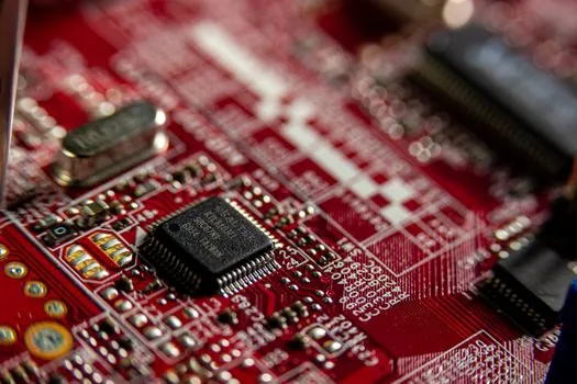
Analog-output 4-20 mA HART transmitters and FOUNDATION Fieldbus or PROFIBUS PA devices run the same CJC algorithm; the difference is that digital-bus units can also publish the cold-junction temperature and raw millivolt as separate variables, which is invaluable for diagnostics and for HART 7/IO-Link asset-management tools that flag a failing reference sensor before the process variable drifts noticeably [S2][S6].
Handheld calibrators like the Fluke 754 perform an equivalent compensation when measuring a thermocouple: an internal thermistor monitors the terminal block and the firmware applies the same NIST polynomial correction, which is why a field calibration loop should always include the transmitter's own CJC in the uncertainty budget [S2].
How to verify compensation in the field
Two practical tests: first, the ice-bath substitute, where the thermocouple wires are shorted together with a copper jumper at the transmitter terminals and the local ambient is measured independently with a calibrated reference probe; the transmitter should read that ambient temperature within its stated CJC accuracy [S1][S4].
Second, the gradient test, where the transmitter is subjected to a controlled 50 °C ambient while the thermocouple input is held at 0 °C (ice bath or electronic mV simulator referenced to 0 °C); the reading should stay within the published ambient-effect coefficient, typically ±0.05 °C per °C of ambient change, and any larger drift usually points to a degraded reference sensor or a loose terminal screw breaking thermal contact with the isothermal block [S2][S4].
For more on how the front-end signal chain interacts with plant control and protective enclosures, see the write-ups on temperature transmitter architectures and how field-side devices sit inside explosion-proof junction box wiring practices. A related spec-deep dive on adjacent sensing hardware, including how IEPE-style two-wire conditioning differs from thermocouple front ends, is in the IEPE charge-amplifier sensor article.
Component reference pages worth checking: reactive power compensation.