A 30-second machine cycle governed by a PLC with a 30 ms scan produces roughly 2,250 fewer parts per year than the same cycle governed by a 6 ms scan, and on a $1,000 part that is over two million dollars of annual margin left on the table [S1].
That delta comes from the basic structure of a PLC scan: input read, logic solve, output write, repeating every few milliseconds, with the controller only able to detect a completed step and start the next one on a scan boundary, so every step transition absorbs at least one full scan of dead time [S1][S3].
Why a Few Milliseconds Per Step Add Up to Real Tonnage
Each scan consists of three phases: input scan (read sensors and module status), program execution (solve ladder, structured text, or function-block logic), and output update (drive actuators, valves, and motor starters), and the total of those three phases is the scan time, normally quoted in milliseconds [S3][S7]. A six-step discrete machine has six such boundaries per cycle, so a 30 ms scan burns about 180 ms per part in transition latency versus about 36 ms at 6 ms, a difference of roughly 144 ms per part that is invisible on the HMI but compounds across millions of cycles [S1].
The same arithmetic scales with cycle length and step count: an engine plant that migrated from legacy controllers to a current-generation processor with lower scan time recorded 120+ additional engines per day, with no mechanical change, no new tooling, and no extra shifts [S1]. On a 30 s cycle running 8 h/day, going from a 50 ms scan to a 30 ms scan also produces a measurable throughput delta, on the order of 2,250 additional parts per year on a single machine, which is why scan time is one of the first things a process engineer audits when a line is underperforming its nameplate [S4].
What Actually Drives Scan Time in a Working Machine
Scan time is a function of instruction count, instruction complexity, the number and type of I/O points serviced, and the communication load on the processor, not raw CPU clock speed alone [S2][S3]. Four levers dominate in practice.
Program size and logic density: every additional rung, every nested conditional, every function block adds execution time, and on a tightly tuned machine the bulk of scan is logic, not I/O [S2][S3]. I/O count and protocol: each discrete and analog point on a slower backplane (legacy Modbus RTU, remote I/O over serial) is serviced sequentially inside the scan window, so compact I/O blocks and modern industrial Ethernet (EtherNet/IP, PROFINET) cut I/O phase duration [S3]. Communication load: HMI/SCADA polling, OPC UA tag subscriptions, and peer-to-peer message instructions all consume scan time, and a poorly tuned SCADA poll at 50 ms on a controller with a 20 ms scan can effectively double the apparent cycle [S3][S6]. Memory and data handling: large recipe arrays, historical buffers, and string handling for barcode or label data are surprisingly expensive on a scan-by-scan basis, and trimming unused tags is one of the higher-return optimizations available without new hardware [S3].
Selecting a Scan-Time Target for a Given Machine

There is no universal "correct" scan time; the right number is set by the fastest event the PLC control loop must catch, the mechanical cycle, and the safety class of the application. Three benchmarks cover most cases. [S2]
For high-speed packaging, labeling, and indexing (cycle under 200 ms, steps in the 10-30 ms range), target a deterministic scan of 1-5 ms, which is the envelope where motion and registration loops stay closed inside one scan without overrun [S1][S3]. For typical discrete machines (cycle 5-60 s, electromechanical actuators), 10-20 ms is the working band where scan latency is a small fraction of step time and is rarely the throughput bottleneck [S3][S4]. For process skids, batching, and slow sequential logic (cycle minutes or longer), 50-100 ms is acceptable, and pushing lower buys little because mechanical limits dominate the cycle [S2][S5].
Two watch-outs from the field: a scan that is too short relative to I/O settling time produces unstable or "chattering" outputs, so fast-scan is not free [S3]; and a single, well-tuned mid-range controller will usually beat an older flagship running bloated code, so the order of operations is always code, then I/O, then hardware [S3][S4].
Measurement, Optimization, and the 2-Scan Rule
The standard field practice is the 2-scan rule: budget two full scans for any input-to-output reaction, because the worst case is one scan to read the new input and the next scan to apply the new output, and a designer who only budgets one scan will see intermittent faults that disappear when the cycle slows down [S1]. To verify, most modern controllers expose a wall-clock scan-time register (Allen-Bradley SST, Siemens OB1 cycle time, etc.) that the engineer reads via the programming software; the spread between minimum, average, and maximum scan is more diagnostic than the mean, because jitter usually points to a periodic task, a communication interrupt, or a single heavy function block [S3][S4].
Optimization sequence that does not require a hardware swap: segment the program into modular subroutines or periodic tasks so time-critical logic runs in a fast task and housekeeping in a 100 ms or 1 s task, remove redundant and always-true rungs, consolidate I/O into denser modules on a faster backplane, throttle SCADA/HMI poll rates to multiples of the scan, and clear unused tags and unused data blocks [S3]. On older or obsolete controllers, a planned migration often unlocks the biggest single gain, and a disciplined bridge plan keeps the old line productive while the swap is staged; the practical field playbook is laid out in this bridge-and-migration plan for engineers holding obsolete PLCs together until the cutover [S3][S4].
Comparison of Scan-Time Optimization Options
Four options are commonly on the table, and they trade cost, downtime, and gain very differently. [S1]
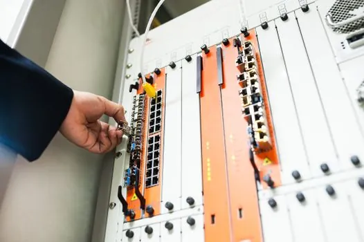
Code refactor: zero hardware cost, zero downtime beyond a controlled download, and the highest ROI when the program has grown organically over a decade [S3]. I/O modernization (compact blocks, industrial Ethernet backplane): moderate cost per drop, single-line shutdown for cutover, and meaningful improvement in diagnostics [S3]. Controller upgrade to a current-generation processor: high one-time cost, planned outage, scan reduction often 4-5x (e.g. 30 ms to 6 ms), and on a high-volume discrete line the throughput gain pays back in months, not years, per the Schneider-Electric calculation cited above [S1]. Network/SCADA retune: low cost, no shutdown, and the right first move when jitter is the visible symptom [S3][S6].
Standards, Sourcing, and Engineering Caveats
Scan time is not a regulated metric, so it does not carry a standard number the way an ATEX or IEC 60079 rating does; what does carry a standard is the safety layer running on top of the scan, where a safety PLC must demonstrably execute its safety task within the application-specific response time the risk assessment demands, and that is a separate, certified timing budget from the standard scan [S5]. Two sourcing rules from the field: vendor-published "typical" scan times assume an empty program and minimal I/O, so real-world numbers are always larger and must be measured, not quoted from a datasheet; and second, identical controllers in the same program can scan at different speeds on different firmware revisions, so any scan-driven retrofit should be qualified on the actual revision that ships to the floor, not the marketing literature [S2][S4].
Two trackable signals to watch: the share of new mid-range controller lines shipping with deterministic multi-task architectures (which lets a fast task carry the throughput-critical logic while a slow task handles housekeeping), and the rollout of OPC UA over TSN on plant networks, which moves more I/O off the scan window and onto a scheduled Ethernet layer, both of which will shift the scan-time-vs-throughput curve in the next hardware refresh cycle [S3].