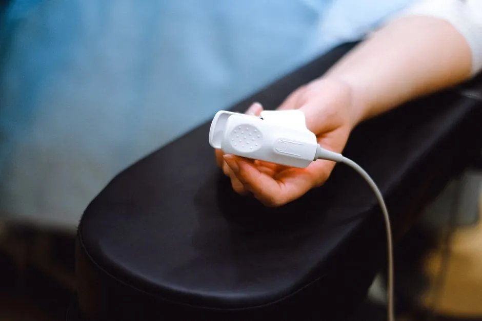
A single transducer fires a short ultrasonic burst (typically 0.5–10 MHz) into the test piece and listens for reflections; the round-trip time between transmit and the flaw echo, divided by two and multiplied by the material's longitudinal sound velocity, gives the flaw's depth below the entry surface [S2][S4].
Depth is read on an A-scan display as the horizontal position of a peak that appears before the backwall echo; once the time-base is calibrated in millimetres for the material under test, every microsecond of echo delay maps directly to a millimetre of metal [S2][S8]. This is the same physical principle that drives a flaw detector on the shop floor and a pressure transmitter shares only a coincidental name, not a technology.
Why a Transducer Doubles as Sender and Receiver
In most pulse-echo systems a single piezoelectric element alternates as transmitter and receiver, with a couplant (gel, water, oil) bridging the acoustic impedance gap between the probe face and the test piece so the sound pulse actually enters the metal [S2][S3]. The piezoelectric disc is damped to ring briefly, typically producing 1–3 cycles per pulse, which gives the system the time resolution needed to separate closely spaced echoes [S4].
Frequencies between 0.5 and 10 MHz dominate industrial flaw detection, with 0.1–25 MHz as the wider UT band, because lower frequencies penetrate coarse-grained steel further while higher frequencies resolve smaller defects, since the generally accepted detection limit for a small flaw is one-half wavelength (λ = c / f) [S2][S4]. For a 5 MHz longitudinal wave in carbon steel, c ≈ 5,900 m/s gives λ ≈ 1.18 mm, so a flaw must be roughly 0.6 mm across to be reliably detected at that frequency [S4].
Converting Microseconds to Millimetres
Depth is calculated with the same relationship a flow meter uses for transit-time, only applied to a solid: d = (c × t) / 2, where t is the measured round-trip interval on the A-scan and c is the longitudinal wave velocity in the material being inspected, roughly 5,900 m/s in steel, 6,320 m/s in aluminium, and 4,700 m/s in nodular cast iron [S2][S4].
Two practical calibration artefacts keep the maths honest: the V1 (or 25 mm) block and the V2 block carry known reflectors at fixed depths, and the operator adjusts the instrument's time-base so the backwall echo from these reference blocks lands at the correct millimetre mark before production testing begins [S4]. Without that step, the absolute depth number is untrustworthy even though the relative echo position still flags the flaw. The same calibration discipline shows up wherever a measurement has to be traced to a physical standard, from a tensile testing machine load cell to a checking and testing apparatus gauge block.
Reading the A-Scan: Flaw Peak vs Backwall Peak
An A-scan plots echo amplitude against time, so the screen shows three landmark signals in a healthy test piece: the initial pulse (t = 0), any flaw echo (intermediate peak), and the backwall echo (final peak); if the operator moves the probe over a defect, the flaw peak grows and the backwall peak shrinks because part of the beam's energy is now reflected sooner [S2][S8]. The horizontal gap between the initial pulse and the flaw peak, read off the calibrated time-base, is the one-way depth of the reflector [S2].
Three structural rules govern what the operator sees on the screen: the flaw echo must arrive after the initial pulse and before the backwall echo, the peak's height roughly tracks the flaw's projected area normal to the beam, and the peak's width is set by the pulse length and the flaw's through-thickness extent, not by its lateral size [S2][S4].
Why Wavelength and Pulse Length Set the Resolution Floor
Two defect peaks can only be resolved when their round-trip times differ by at least the pulse length, and the smallest detectable flaw is about one-half wavelength across, so a 2 MHz probe in steel (λ ≈ 2.95 mm) misses defects under ~1.5 mm while a 10 MHz probe (λ ≈ 0.59 mm) resolves down to roughly 0.3 mm at the cost of higher attenuation and shorter inspection range [S2][S4].
This is why rail axle and subsea-pipe inspection, the same cylindrical components modelled in recent ultrasonic measurement work, use line-focused transducers that concentrate energy along a focal line: the focal geometry raises the signal-to-noise ratio against the curved backwall and improves depth resolution in components where a planar probe would smear the echo [S1]. The selection between contact, immersion, and angle-beam probes follows directly from these wavelength and resolution limits, not from operator preference.
What Pulse-Echo Cannot Tell You
Pulse-echo depth is reliable only for reflectors that face the probe with a normal component; a crack oriented parallel to the beam reflects almost nothing back and the flaw either disappears or returns an amplitude so low the operator mistakes it for background noise, which is why angled (shear-wave) probes are specified for transverse crack sizing on welds and pipelines [S2][S5].
Coarse-grained austenitic stainless, thick concrete, and heavily attenuating composites all push the detection limit past the half-wavelength rule because grain scatter raises the noise floor, and operators fall back on B-scan or C-scan imaging, where many transmit-receive pairs are combined into a cross-sectional image showing depth and lateral position simultaneously, when the single-channel A-scan no longer separates flaw from structure [S7]. Inline inspection crawlers used in gas and liquid pipelines add a tilted pulse-echo arrangement precisely because 0° pulse-echo cannot reliably detect crack-like features [S5].
Comparing the Three Common Pulse-Echo Configurations
For depth measurement on a typical shop floor, the three practical configurations line up as follows against four decision criteria: single-transducer pulse-echo (1) on a contact probe gives the simplest setup, full depth range, resolution limited to ~½λ, and works only when the defect face is roughly normal to the beam; pitch-catch with separate send and receive transducers (2) doubles the inspection zone, suits curved or limited-access geometry, and improves signal-to-noise on attenuating materials; and angle-beam shear-wave pulse-echo (3) detects tilted cracks that a normal probe misses, trades some near-surface resolution for oblique coverage, and is mandatory for weld and pipeline-crack sizing to standards such as ASME V Article 4 and API 5L inspection practice [S2][S3][S5].
Choosing between them comes down to four questions: what orientation will the defect present, how deep is the zone of interest, what is the grain structure of the alloy, and is the inspection point automated (immersion) or hand-held (contact). The same selection logic is documented in operator training for any industrial valve pressure-containing inspection, where defect orientation, base material, and access geometry decide the technique before the probe ever touches the part.
Track two signals going forward: the migration of phased-array and total-focusing-method (TFM) imaging into handheld flaw detectors, which improves depth-sizing accuracy on coarse-grained welds beyond classical pulse-echo limits, and the continued certification of inline pulse-echo crack tools that have logged inspection runs exceeding 1,000 miles of pipeline on a single campaign [S5]. Operators calibrating against IIW V1/V2 reference blocks and following ASME V or EN 12668-1 instrument standards will see the most consistent depth numbers, regardless of whether the probe is 2 MHz or 10 MHz.
This topic is covered further in PNP vs NPN Proximity Sensors: Sensing Range Holds, Output Logic Decides.