
A machine vision system pairs industrial cameras, optics, structured lighting, and embedded or PC-based image processing to inspect hundreds to thousands of parts per minute, with throughput governed by sensor resolution, frame rate, and exposure control [S2].
The global machine vision market is projected to grow from $15.83 billion in 2025 to $23.63 billion by 2030, and that widening vendor pool is exactly why a written specification, written before any demo, is the single most valuable artifact in the buying cycle [S5].
Scope: What Counts as a Machine Vision System
Machine vision is the industrial subset of computer vision, engineered for deterministic latency, ruggedised enclosures, and direct integration with PLCs, robots, and MES layers, not for general image recognition [S2].
Every system breaks into five functional blocks: image acquisition (camera, lens, vision light source, frame grabber), image processing and recognition (algorithm plus compute), result output, system control, and a display/HMI layer [S2]. The OPC UA companion specification OPC 40100-1 standardises an information model across those blocks with object types for VisionSystem, ConfigurationManagement, RecipeManagement, and ResultManagement, so a cell can publish structured results and accept recipe changes from a MES without custom drivers [S2].
The Four Selection Gates: Resolution, Throughput, Environment, Integration
Resolution and sensitivity are the two governing sensor specifications: higher pixel counts enable detection of smaller features for electronics, pharmaceutical packaging, and semiconductor work, while higher sensitivity keeps detection reliable at low contrast or high line speed [S1].
Cycle time is the second hard gate, and a useful rule of thumb from the research: a line that must inspect hundreds or thousands of parts per minute cannot run on a smart camera limited to a handful of frames per second, while a slow manual station has no business with a 10 GigE multi-camera rig [S1]. Third is environment: an automotive weld cell sees spatter, EMI, and thermal swings that a cleanroom tool does not, so IP65+ housings, ruggedised lenses, and filtered light source drives are non-negotiable. Fourth is integration, where OPC UA, GigE Vision, PROFINET, and EtherNet/IP support on the datasheet matters as much as megapixel count [S1].
Sizing the sensor follows two numeric rules: aim for at least 2-3 pixels across the smallest rejectable feature, and pair resolution with frame rate matched to line speed, then confirm a global shutter to suppress motion artefacts on moving parts [S2]. For 2D area work, 5-20 MP sensors are standard on electronics and pharma packaging lines; for continuous webs, 2K-16K line-scan sensors are used at line speeds above 10 m/s [S2].
Smart Camera vs. PC-Based Multi-Sensor: The Architecture Decision

The architecture choice is governed by cycle time, number of inspection points, and environmental sealing, not by software brand, and a smart camera will not survive any RFQ where throughput, deep-learning inference, or multi-camera synchronisation is on the requirement list [S2].
Comparison of the two realistic options across four engineering criteria, drawn from the research:
Cycle time: smart cameras typically handle 10-100 inspections per second on simple presence/absence, barcode, or 1D/2D code reading tasks, while PC-based multi-camera systems sustain hundreds to thousands of parts per minute when paired with GigE Vision or 10 GigE bandwidth and FPGA or GPU inference [S1][S2]. Integration cost: smart cameras win on lowest integration cost, a single IP address, and factory-calibrated optics, but they lose on processing headroom, fixed I/O count, and the inability to add a second camera or a higher-power vision light source [S1]. Environment and cyber: a sealed smart camera shrinks the OS-patching and cyber-attack surface; a PC-based system brings more cabinet space, more patching, and a larger attack surface, but unlocks deep-learning inference and 2D/3D fusion [S1]. Best fit: smart camera for standalone stations; PC-based multi-sensor for high-speed electronics, pharma blister packs, and any duty requiring fused 2D/3D results [S1].
Sensor Class: 1D, 2D, 3D, and Spectral
Machine vision systems are categorised into four technology classes, 1D, 2D, 3D, and spectral or colour imaging, and the choice is driven by what must be detected, not by camera brand [S2].
A 1D system reads barcodes, lot codes, and continuous web defects at the highest line speeds; a 2D system handles pattern matching, OCR, and surface inspection; a 3D system delivers height maps via laser triangulation, structured light, or time-of-flight; a spectral system separates materials by reflectance or fluorescence [S2]. For buyers, that means the sensor class is a function of the defect catalogue, not the vendor shortlist.
Camera-Level Pitfalls: Shutter, Lighting, and Bandwidth
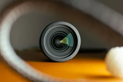
For robotic guidance, where the camera is mounted on a moving gantry or in an eye-in-hand configuration, rolling shutter distortion corrupts not only the appearance of the target but also the computed pose used to drive the motion planner, and that positioning error compounds over successive picks, which is why global shutter is a baseline requirement rather than an optional upgrade in that application class [S3].
Lighting geometry is the second most common source of false rejects: directional lighting that creates shadows or specular glare confuses edge-detection algorithms, while diffuse or structured lighting produces the uniform contrast that modern software models expect, and engineers who lock the lighting design with the vision software vendor before RFQ see fewer false rejects in the first months of production [S3]. On bandwidth, the practical guidance from the field is to balance cable routing constraints against the bandwidth the inspection task genuinely requires, and to resist over-specifying bandwidth just because a vendor recommends it [S3]. Global shutter sensors do carry a price premium tied to more complex pixel architecture, although the gap has narrowed with stacked-sensor designs, and at very high resolutions the price delta can still be substantial, so it pays to compare specific models rather than assume a fixed markup [S3].
Writing the Inspection Specification Before the Demo
A specification that defines minimum defect size, required recall rate, line speed, and data integration requirements turns every vendor demo into a pass or fail test, and the cost of skipping this step is measured in weeks of vendor management time and recurring false-reject tickets after the PO [S5].
The specification should answer five questions: defect types and minimum detectable sizes, with physical examples and surface conditions; required False Acceptance Rate and False Rejection Rate, with FA = 0% and FR ≤ 1% as a typical deployment target; line speed and available inspection window, where a 400 mm/s line on a 100 mm part leaves 250 ms per part, of which the AI inference budget is typically under 50 ms after PLC trigger latency and reject mechanism response; mandatory integration points, including PLC protocol and MES receivers; and the lighting and mounting constraints that will be imposed on the cell [S5]. Buyers who anchor on these numbers before talking to vendors also avoid the more common trap noted in the field: systems that require cloud inference for production decisions, or cannot reliably trigger reject mechanisms within the part dwell time, will not function on high-speed lines [S5].
Standards, Compliance, and Supplier Comparison Anchors
International standards such as ISO 9001:2015 for quality management and ISO 13485 for medical devices often reference vision system capabilities, while EMVA 1288 provides a unified method for measuring and reporting camera performance, which is critical when comparing suppliers across regions [S4].
For supplier comparison, the practical anchors from the field are: speed, with industrial machine vision rated up to 1000+ parts per minute versus 30-60 ppm for fatigue-limited manual inspection; accuracy, with sub-micron level achievable under proper calibration versus a typical 85-95% accuracy band for human inspection; initial station cost in the $5k-$50k range depending on configuration; and compliance, where machine vision systems can be specified to meet FDA 21 CFR Part 11 electronic-records and signature requirements, a difficult bar for manual stations to clear [S4]. A typical deployment replaces 3-5 inspectors per shift, runs 24/7 without fatigue, and feeds digital logs directly into MES or ERP for SPC and traceability [S4].
Procurement Signals to Track Before Issuing the PO
One practical spec-first rule distilled from the research: if any of (a) throughput above 50 fps, (b) more than 2 cameras per station, (c) deep-learning inference, (d) OPC UA recipe exchange, or (e) IP65+ rating is on the requirement list, the buyer should be pricing a modular controller plus separate camera systems from day one, not a single-box smart camera [S1].
For a related walkthrough of how a spec-first cell gets built for a different inspection duty, see this labeling machine selection playbook for automotive parts logistics, which applies the same defect-class-plus-throughput-first logic to a print-and-apply cell. Buyers evaluating cooling for the vision cabinet or the line-side industrial PC will find the immersion cooling sourcing map useful for thermal budgets on dense GPU inference racks, and the UPS topology map for China sourcing covers the ride-through spec that any PC-based vision controller inherits by default. Trackable signals worth recording on the next sourcing cycle: vendor disclosure of which OPC UA companion specification profile they implement, the latency budget from trigger input to reject output measured on the buyer's actual line, and the sample-efficiency claim demonstrated live against the buyer's own defect samples rather than a vendor benchmark [S2][S5].
Component reference pages worth checking: machine vision id, and vision measuring machine.